Large-Scale Distributed Sentiment Analysis with RNN
Model Design
Click here to go back to Homepage.
The entire model is a 2 step process - the first one involves preprocessing the data using MapReduce, and the second one parallelizes Recurrent Neural Network on multiple GPUs using PyTorch CUDA+NCCL backend. AWS has been used for flexibility to test tradeoffs for different number of GPUs, nodes and different kind of GPU models.
Table of Contents
I. Data and Preprocessing
I.0. Data Description
In this project, we use raw Amazon product review data from [1] and [2]. This public dataset consists of 142.8 million product reviews along with the corresponding ratings, reviewer IDs, product IDs, and other information, spanning from May 1996 to July 2014. It is suitable for our project because we can use the rating as a proxy of the sentiment in the review. Review data are quite abundant that we would need distributed algorithms to match our needs to process the data and perform the analysis in a reasonable amount of time.
I.1. Serial Version
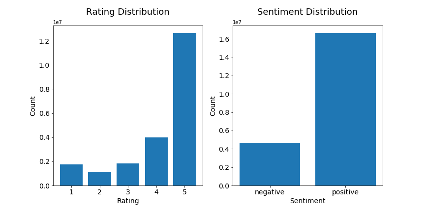
The first preprocessing step is to remove duplicates of text, in order to reduce unnecessary noises as well as to shrink data size. Because our project focuses on analyzing the sentiments within text, reviewer and product information is irrelevent. Thus, we remove duplicates only by the content of the review. Repeated text often have different ratings, and we only keep the one that appears the most. When there is a draw in frequency, we keep the one of smaller rating score with the intention to balance the dataset, since we find that a majority of the reviews already have ratings of 5. After removing duplicates of text, we are left with 21.3 million distinct reviews.
The ratings have a range of 1 to 5, and the distribution is illustrated in the histogram below. We combine 1, 2, and 3 into negative sentiment, and we combine 4 and 5 into positive sentiment. The distribution after such grouping is also illustrated below.
Second, in order for RNN to process our data efficiently, we need to remove stopwords (words with little contribution to sentiment classification) and map the other meaningful words to numbers. The stopwords are inherited from the nltk package, and we add additional stopwords like ‘product’, ‘would’, and ‘get’. The word-number dictionary are generated from our own dataset, in which only the most frequent 10,000 words are kept. Words not included in this dictionary are mapped to a specific number indicating ‘unknown’.
Lastly, the input to our RNN needs to have a fixed length, which we set to be 100. After the removal of stopwords, sequences that are too long are truncated, and sequences that are too short are padded.
I.2. Parallelization
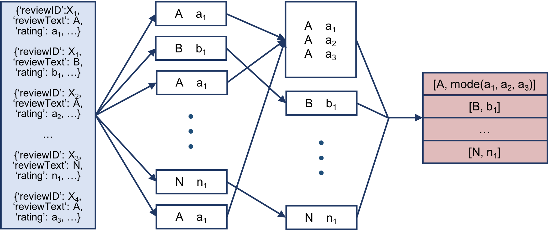
The data preprocessing task is parallelized through MapReduce. The mapper reads in the raw data, removes special characters from the text, and outputs only the text and the ratings. The reducer reads in the output of the mapper, sorted first by the text, so that repeated texts are together. It further processes the text (remove stopwords, map words to numbers, and truncate or pad to achieve ideal length). Furthermore, it calculates the mode of ratings for each distinct review text and maps it to 0 or 1 to indicate negative or positive sentiment. This sentiment indicator value is appended to the end of the text sequence, and the output is written as a numpy array.
One of our biggest challenge is how to store the processed data to allow efficient writing and reading without blowing up the memory. We considered json and pickle, but they both have the problem that if we try to read from the file, we need to first load the content of the entire file. We also considered saving each text sequence in a separate file, but that introduces extensive communication overhead during RNN training. Thus, we choose to save our data as chunked datasets in an hdf5 file. The benefit is that the program only loads the small chunks of data that we specify by dataset key and chunk index.
Because our dataset is so large, we perform the MapReduce process on an AWS EMR cluster. The cluster reads data from an S3 bucket. In order to prevent overwriting the results, each worker node generates a separate h5 file and uploads it back to the S3 bucket, and the files are differentiated by including the host name of the node in the file name. We found that best performance is achieved through having 8 m4.xlarge worker nodes in the cluster.
We combine these intermediate h5 files into one single file on an m4.2xlarge EC2 instance so that it has larger memory to handle large arrays. Again, to avoid exceeding the memory limit, in this final h5 file, data from each intermediate file is grouped in one dataset, and each entry of data (a pair of word sequence and sentiment indicator) is stored as a chunk.
II. RNN Model
II.1. Serial Version
Due to serial nature of customer reviews, we use Recurrent Neural Network to model the time dependency of words in each sentences and predict whether the review is positive or negative. We apply LSTM layers instead of regular recurrent neural network because it is more robust to vanishing or exploding gradient problems. We trained an embedding layer to reduce the dimensionality of word representation. Hyperparameters such as number of layers and hidden dimensions are tuned on our dataset, with careful consideration for the tradeoff between model performance and compuational time.
Our dataset is highly imbalanced, with 12 million 5-rating review, accounting for 59% of the data. After recoding scores into 2 sentiment class for more general interpretability, the positive class is still overwhelming in size. To overcome this imbalance, we experimented with multiple loss functions such as MSE (recoding response as continuous), crossEntropy and BCEWithLogitsLoss. We chose loss function to be BCEWithLogitsLoss because it is both numerically stable and has the flexibility to incorporate class weights. The dataset class breakdown before and after this change is reported in details in our data section.
II.2. Parallelization
Recurrent Neural Network is parallelized through PyTorch Distributed Data Parallel module with CUDA, using NCCL backend (an MPI-interface) for multi-GPU communication as shown in the diagram below. And the data loading process is parallelized through PyTorch Distributed Sampler module, which assign each node deterministically its own portion of the data using a random seed equal to the current epoch. This avoids the need of communicating the split of data across each node. In addition, multiple cores have been used to load the data through PyTorch wrapper from the native multiprocessing module, as the amount of data to load is quite large for a single core to handle.
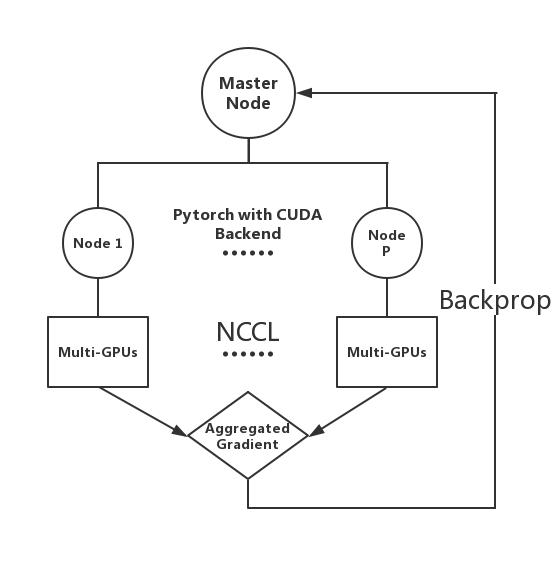
The parallelization is carried in a SPMD (single program multiple data) manner. At first, each GPU gets its own share of the data by determining its split deterministically. For instance, for 2 nodes first one takes the fist half of a shuffled data based on a random seed equal to the current epoch. Then, via NCLL the model is replicated on all GPUs to keep a single program. During the forward and backward propagation, each GPU calculates its own loss and the corresponding gradient. The gradients are first divided by the batch size and then sum reduced together and averaged to get the corresponding averaged gradient. This gradient is propagated back to all GPUs so that the update would result in the same model. This process is repeated until convergence. Most of this process has been wrapped by PyTorch distributed modules, but the knowledge of its mechanism is necessary for us to implement our own dynamic load balancing and merge it seemlessly with Pytorch interface.
Given how this is both a GPU (computing the network weights) and CPU intensive task (loading the data), we parallelize this with multiple nodes to gain access to multiple GPUs and processors, by launching a GPU cluster on AWS. As G3 instance (8 physical CPUs) contain more processors than P2 (4 physical CPUs), we choose mostly G3 for our experiments. AWS has been used for the flexibility to customize with different setups.
Finally, to save cost on storage and to prevent from downloading multiple copies of the data, we share the data folder through Network File System (NFS).
II.3. Advanced Feature
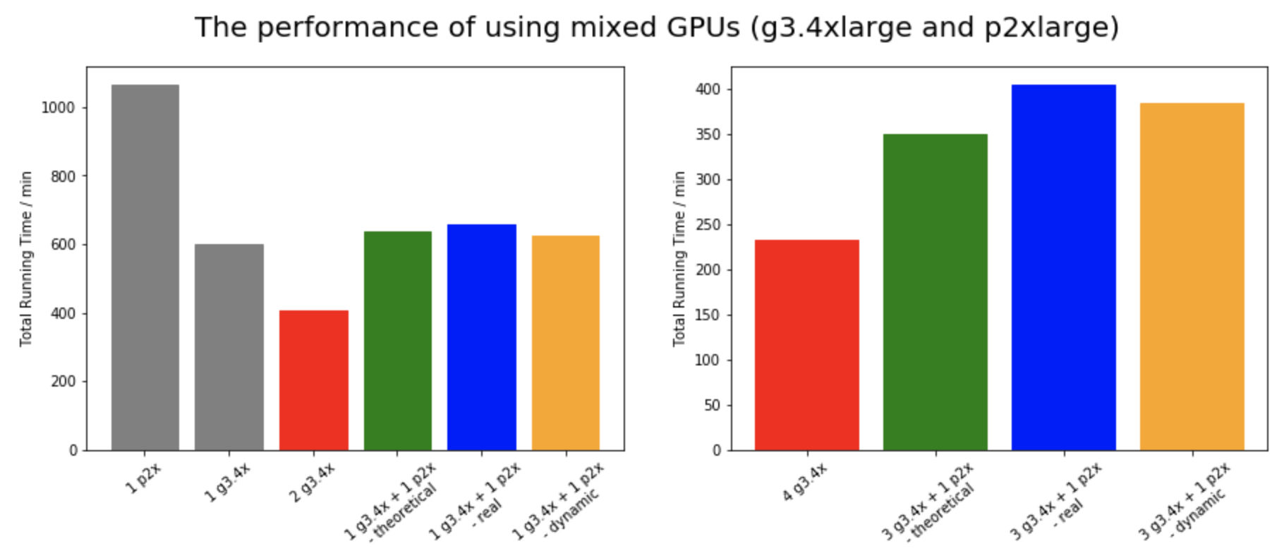
Besides the Bootstrap Actions on MapReduce and parallelizing a neural network on PyTorch (topics not taught during the course), we also implement a dynamic load balancer for the neural network to augment existing data loader and distributed data sampler modules. Looking at the PyTorch distributed source code, we realized that PyTorch distributes the same batch size and amount of data for each GPU indiscriminately. This would introduce a huge bottleneck for a mixed GPU setup or when some GPUs are slower than others due to thermal cooling or other uncontrollable traffics. This bottleneck is caused by the fact that at the gradient aggregation step, we need to wait for all GPUs to finish forward and backward propagations to synchronize - this would result in a huge load imbalance if there is one GPU much slower than the rest. In fact, the graph below shows that when mixing GPUs, the performance drops drastically compared to using a cluster of same GPUs.
To mitigate this load imbalance, we create our own dynamic load balancer that readjusts the distributed data loaders for each GPU to redistribute the portion of data and the correponding batch size based on the forward runtime. The following diagram illustrates this concept for 4 nodes with 3 g3.4xlarge and 1 p2.xlarge instance.
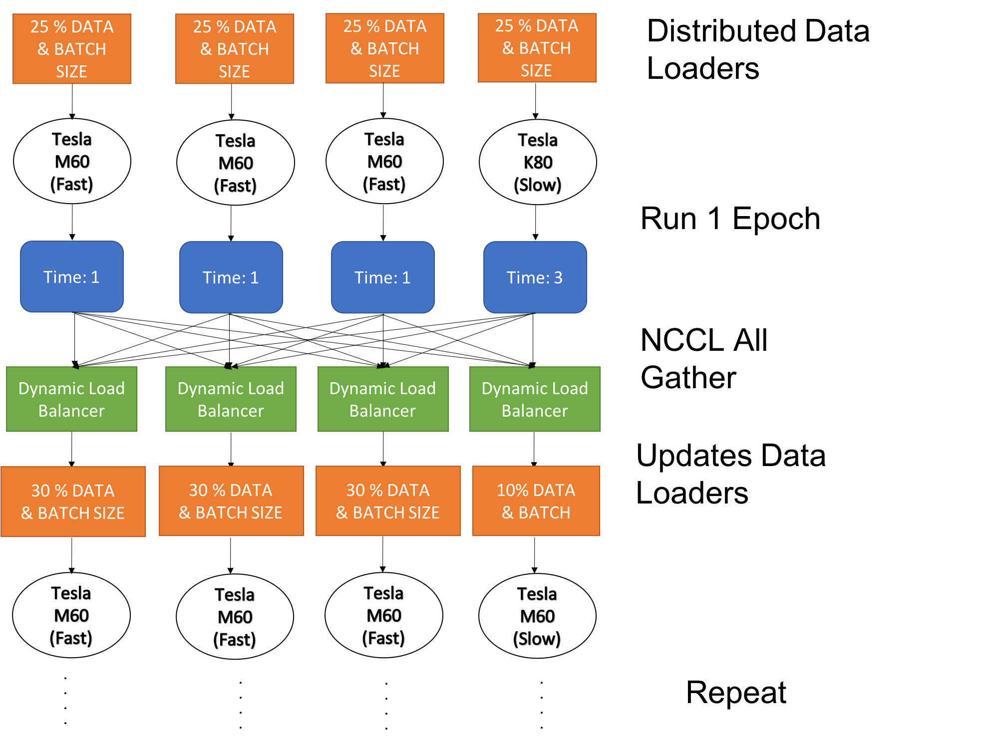
Each GPU starts off with evenly distributed portions of data and batch size, as we do not know how fast each one is at first. After running one epoch or every X epoch (as defined by the user in the input argument), the forward runtime is gathered from all the GPUs and passed to the dynamic load balancer. The dynamic load balancer uses the that runtime to estimate how fast each GPU is and instantiates a new data loader with the newly distributed portion of data and batch size, replacing the old distributed data loader. In this way, the workload of each GPU is readjusted. Note that the both the amount of data and batch size have been adjusted accordingly so that the total number of iterations on each GPU matches to prevent issues such as communication deadlock where one is waiting for synchronization when another one has already finished its iterations. To implement this dynamic load balancer, we have augmented the Distributed Data Sampler from PyTorch to keep track of data split and percentage of data for re-updating the load estimates.
Please see Performance Results for the improvement from using dynamic load balancer.