Experiments and Performance Results

Click here to go back to Homepage.

Metrics of Performance
Data Preprocessing
- Overhead and Mitigation Methods
- Performance Analysis
Running SGD with RNN for Sentiment Analysis

I. Metrics of Performance

While measuring the performance in terms of parallelization, we focus on the following metric:

Throughput: Throughput is defined as the ratio of problem size to the running time.
Speedup: In general, speedup is a number that measures the relative performance of two systems processing the same problem. Specifically, if the amount of time to complete a work unit with 1 processing element is t1, and the amount of time to complete the same unit of work with N processing elements is tN, the strong scaling speedup is t1/tn. Also, under the weal scaling setting, t1 and tn are both measured with different total problem size (same size for every node), i.e., t1 will change with the number of processor, Then the weak scaling speedup is calculated correspondingly. Note the definition of weak scaling speedup is usually obscure, here we use this definition.
Efficiency: Efficiency refers to the ratio of the speedup to the number of processors, which is ideally constant.

II. Data Preprocessing

Overhead and Mitigation Methods

The main overhead comes from sequential code. First, to remove stopwords, we need to compare each word in the sequence with intended stopwords to determine whether we remove this word from the sequence. We save the stopwords in a set instead of a list to shorten the runtime from O(N) to O(1). Moreover, when we combine the h5 files, it takes a long time to write data to h5 files, especially when we save as many different datasets within the h5 file. Ideally, we would want to save all data in one single h5 dataset. However, we need to save data in a single array before saving it as a dataset, and we are restricted by the memory size of the instance. Therefore, we decide to save data into eight separate datasets with equal size. For faster reading during the training process, the datasets in the h5 file are chunked, so that when the data loader accesses a single entry, it does not need to load any other data into the memory.

A second source of overhead is communication. To avoid overwriting, each node in the EMR cluster writes its own h5 file and uploads to the S3 bucket. This time is reduced by having multiple nodes process the data and each upload a section of processed data at the same time.

Performance Analysis

The runtime with different problem sizes and numbers of processors is listed below:

Percentage of Full Dataset	Runtime with 2 Nodes Cluster	Runtime with 4 Nodes Cluster	Runtime with 8 Nodes Cluster
25%	99 min	28 min	14 min
50%	Failed	51 min	30 min
100%	Failed	Failed	55 min

We simply were not able to process more than 1/8 of the data on one single node because the worker nodes get unstable. Even when we tried to process 1/4 of the data on a two nodes cluster, the runtime is abnormally long. Therefore, we are not able to calculate metrics like speedup under week scheduling setting, and speedup under strong scheduling setting is calculated against runtime on two nodes.

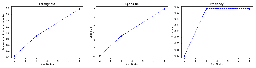
Under Strong scheduling setting, the metrics with fixed problem size (25% of the data) are calculated as follows:

Under the idea of weak scheduling, the runtime with fixed problem size per node is illustrated below:

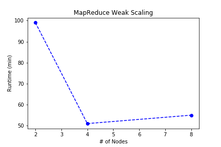
We observe roughly linear speedup and throughput with fixed problem size. We suspect that the runtime for 25% data on two node cluster is abnormal, so the relationship should be more linear, and the efficiency should be similar. Moreover, the runtime for fixed problem size per processor should be similar, as well.

III. Running SGD with RNN for Sentiment Analysis

Since AWS does not approve our request of 8 g3.4xlarge instances, we can only use 4 g3.4xlarge instances (each with 1 GPU) and 2 g3.16xlarger instance (each with 4 GPUs). Along with limited credits, our experiment results would be a little bit biased and limited due to different memory, network, I/O and configurations, etc.

Code Baseline

We run sequential RNN on 1 g3.4xlarge instance, which would be our code baseline. Results are shown below:

epoch	time(s)	test acc	test f1
1	3840	81.41%	0.85
2	3542	83.48%	0.86
3	3572	83.59%	0.86
4	3570	83.73%	0.86
5	3605	84.36%	0.86
6	3534	84.29%	0.86
7	3564	84.22%	0.86
8	3564	84.76%	0.86
9	3544	84.43%	0.86
10	3573	84.96%	0.86

Total training time: 9.98 hours

Also, we profile this code, whose profiling results are shown below:

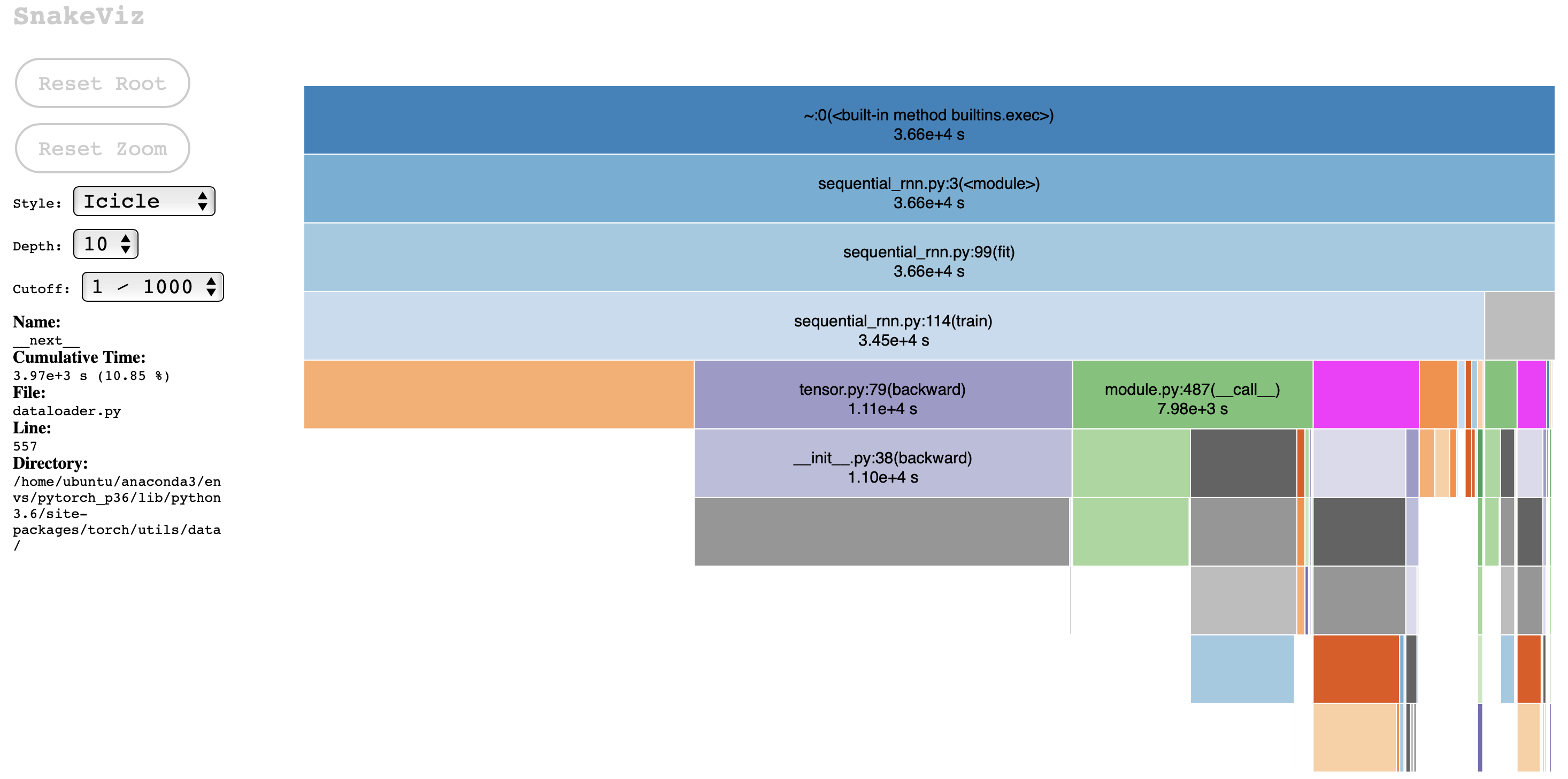
From this profiling result of a single g3.4xlarge instance, we see that this is mainly a GPU intensive task where tasks such as, backward and forward propagations, take up to 50% of the entire run time. This is also somewhat CPU intensive in that data loading takes about 10% of the runtime. Therefore, we should mainly focusing on parallelizing the GPU aspect and its overhead while reducing the data loading process through multi-core parallelization whenever possible.

Experiment with different number of GPUs

In order to see whether our model is strongly scalable, we run our model on the whole dataset with different number of GPUs. Specifically, we tried 1 GPU (1 g3.4xlarge instances), 2 GPUs (2 g3.4xlarge instances), 4 GPUs (4 g3.4xlarge instances) and 8 GPUs (2 g3.16xlarge instances). The results are shown in the following figure:

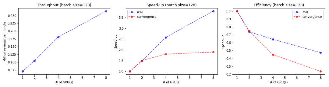
Consistent with Facebook’s paper, we can see the linear throughput and log-linear speed-up. However, the efficiency decreases as the number of GPUs increases, which indicates our model is not strongly scalable. Further, here we calculate the speedup and efficiency in terms of two “time” - real execution time for 10 epochs and convergence time when loss is below 0.13. These two measurments of time both have practical meaning since we are concern with how long each epoch takes and how long the covergence requires. We find that the speedup and efficiency is calculated based on the convergence time is lower, which is reasonable since data parallelism can slow up convergence.

Also, we investigate into the convergence of our RNN with different number of GPUs. In terms of the number of epochs and execution time, we set the loss value 0.13 as the convergence threshold, and obtain the results as follow:

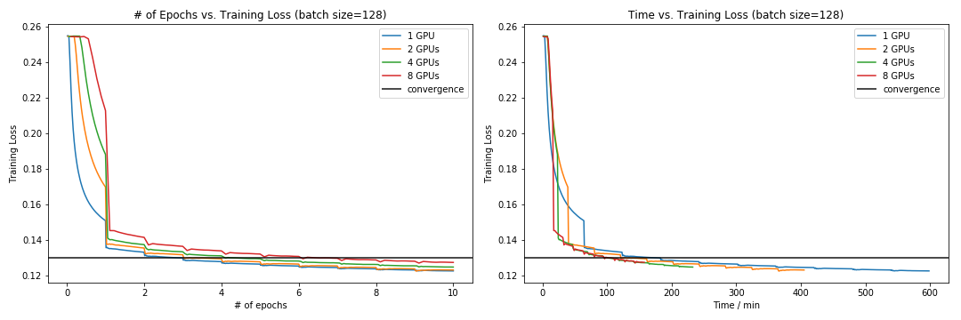
The results exactly match our intution:

The principle of parallel SGD and its convergence is based on Gradient Aggregation. Basically, the aggregated gradient is used to approximate the true gradient, and when the number of epochs increases, this approxmation becoomes precise. Also, from the left plot, in terms of the number of epochs, we can see that 1-node version has highest rate of convergence, and 8-node version has lowest rate of convergence.
While the number of GPUs increasing, each GPU will handle a smaller part of data, which means the time of each epoch decreases. Also, the advantage of Gradient Aggregation is that the approxmation of gradient can be attained more quickly. From the right plot, in terms of the running time, the model with more GPUs converges faster, which suggests the convergence is accelerated by data parallelism.

Experiment with different distribution of GPUs

We also experiment our model when the total number of GPUs is fixed. Specifically, with total 4 GPUs, we ran our model on 1 node with 4 GPUs (1 g3.16xlarge instance), 2 nodes with 2 GPUs (2 g3.16xlarge instance, each only use 2 GPUs) and 4 nodes with 1 GPUs (1 g3.16xlarge instance). The results are shown in this table:

# of Node	# of GPUs per Node	Time (min/epoch)	Speed-up
1	4	21.9	2.73
2	2	26.4	2.27
4	1	23.3	2.57

We can see that 1-node-4-GPU version has best speedup and 2-node-2-GPU version gives the worst speedup. Also, we assess each model’s covergence, which are shown in the following plot:

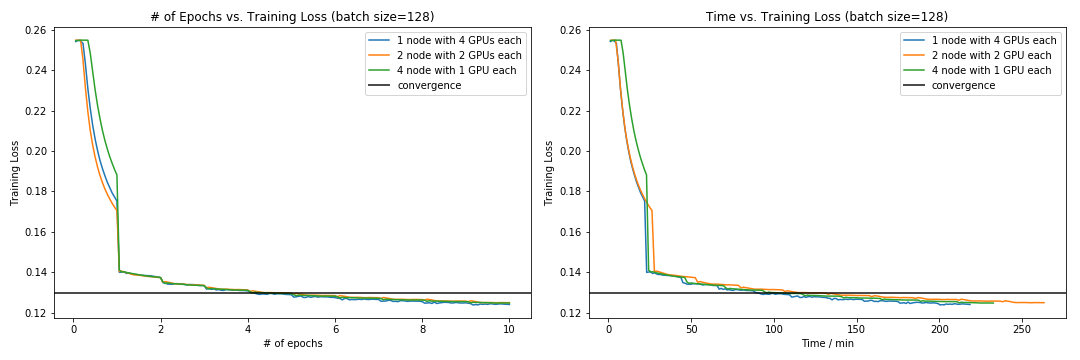
This plot shows that these three version has same convergence rate, except that the loss 4-node-1-GPU version decreases slowly at first. Perhaps it is becuase the communication overhead, but also can be the stochasticity introduced by SGD.

Experiment with different problem size

In order to show weak scaling speedup and efficiency, we randomly sample 25%, 50%, and 100% data and run our RNN model on them with 1 GPU (1 g3.4xlarge instances), 2 GPUs (2 g3.4xlarge instances), 4 GPUs (4 g3.4xlarge instances). The result plots are shown below:

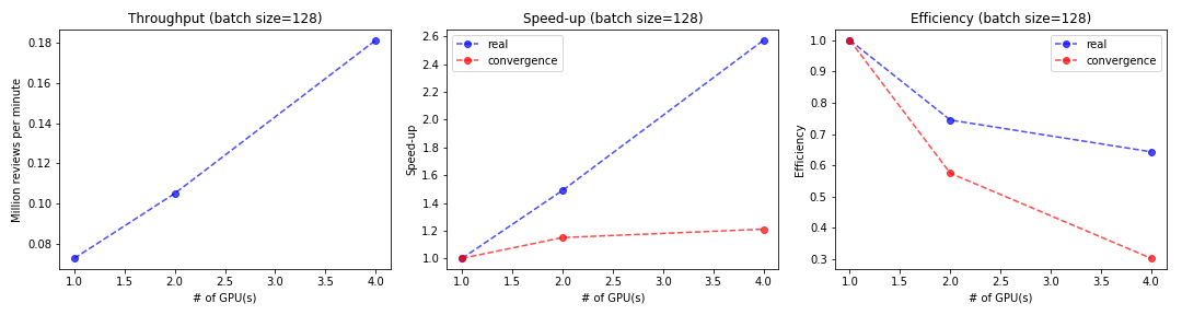
As we can see, the similar results with strong scaling are obtained under weak scaling setting. Thus, our model are also not weakly scalable.

Experiment with mixed of GPUs using dynamic load balancer

As we mentioned in Model Section and demonstrated in the bar plot below, our dynamic load balancer has shown the success while using mixed GPUs (p2xlarger and g3.4xlarger).

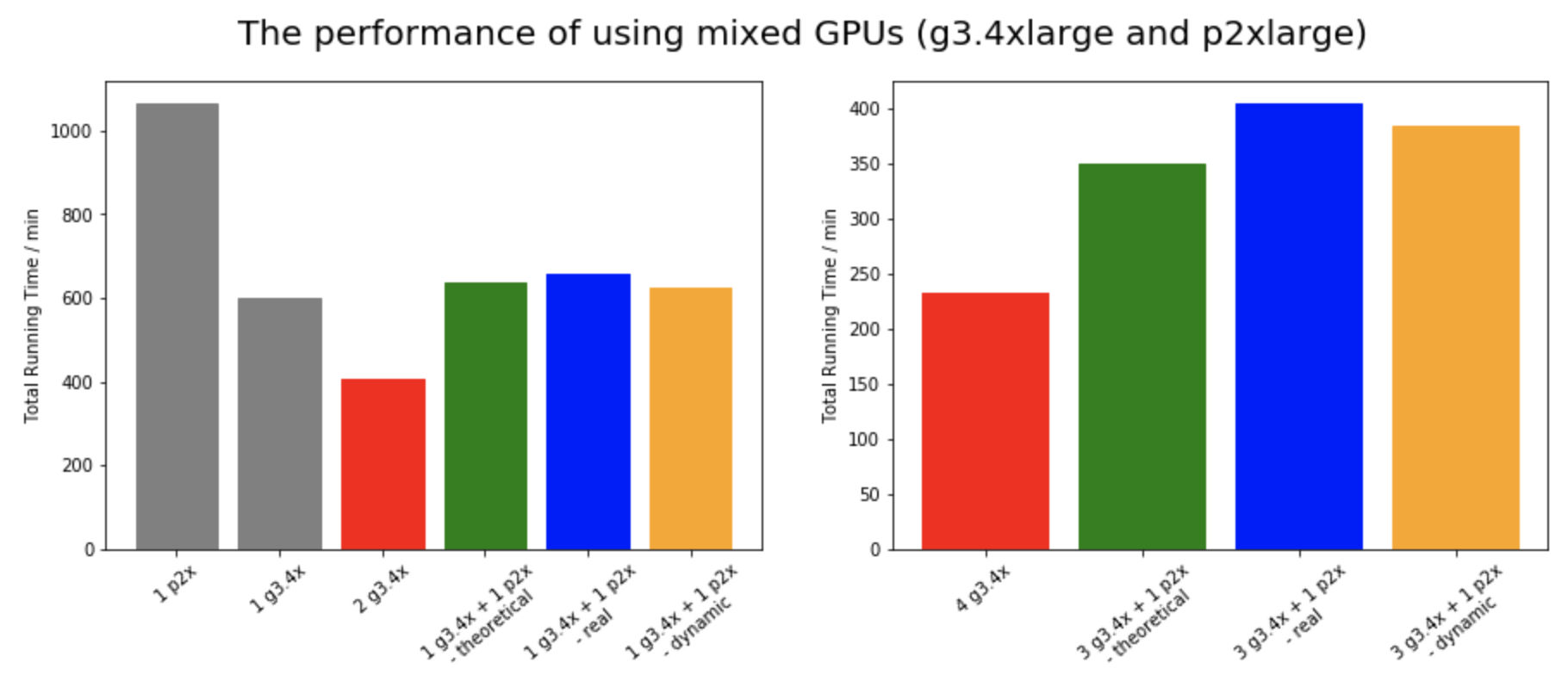
For mixed GPUs setting, we test with 1 p2.xlarge + 1 g3.4xlarge and 1 p2x.large + 3 g3.4xlarge. We also run 2 g3.4xlarge and 4 g3.4xlarge to get an idea what is the rough runtime lower bound that we can achieve, since g3.4xlarge is faster than p2.xlarge. We calculate the theoretical performance by taking into of the difference in performance between one p2 and one g3, and subtract this difference from 2 and 4 g3.4xlarge, our lower bounds. We should hopefully reach the theoretical performance if everything is perfectly optimized. However, this is not reachable in our experiment, since the first epoch is run in imbalanced way to estimate the data split for the next epochs. We’d need to run a large amount of epochs to average out the overhead from the first epoch. Nonetheless, we see that our dynamic balance loader has successfully mitigated this imbalance overhead to an extent, making it faster than the non-dynamic setup for both 1 P2 +1 G3 and 1P2 + 3 G3 setups.

Money-speed Tradeoff

AWS Cost Table:

Instance	Price/hour
p2.xlarge	0.9
g3.4xlarge	1.14
g3.16xlarge	4.56

Table of Total Costs for 10 epochs

Experiment	# p2.xlarge	# g3.4xlarge	# g3.16xlarge	Seconds	Hours	Total Price
Single g3.4xlarge	0	1	0	35920	9.98	11.38
Single p2.xlarge	1	0	0	63923	17.76	15.98
Single g3.16xlarge	0	0	1	13156	3.65	16.64
Two g3.4xlarge	0	2	0	24316	6.75	15.39
Two g3.16xlarge with 2 GPU only	0	0	1	15820	4.39	20.02
Four g3.4xlarge	0	4	0	13973	3.88	17.69
Two g3.16xlarge	0	0	2	9531	2.65	24.17
Three g3.4xlarge + one p2.xlarge	1	3	0	24256	6.74	29.12
Three g3.4xlarge + one p2.xlarge + dynamic	1	3	0	23007	6.39	27.6
One g3.4xlarge + one p2.xlarge	1	1	0	39382	10.94	22.32
One g3.4xlarge + one p2.xlarge + dynamic	1	1	0	37503	10.42	21.26

After running all the experiments, we compile the list of GPUs we have used, the total time taken for each to run 10 epochs and the corresponding costs. From this table, we see that p2.xlarge is significantly slower and more expensive than g3.4xlarge. Due to money and time constraints, we decided to run the rest of the experiments mainly in g3 instances for this reason.

From this table we can conclude that for this distributed RNN:

g3.4xlarge is the cheapest due to no communication overhead but is also quite slow taking up 10hours.
g3.16xlarge is the cheapest one amongst of the fastest ones (less than 5 hours or over 2 speedup), as it only have intranode communication which is lower than internode communication overhead.
Therefore, single node GPUs are usually best money for value given the lower overhead involved. So, you can go for any single node multi GPUs for the best combination of speed and price.
mixed GPUs affect the performance severely with the slowest GPU being the bottleneck, making it a high cost and low performing option. So, avoid this whenever you can.

Large-Scale Distributed Sentiment Analysis with RNN